How We Know The Effect of CO2 on Global Temperature: Part 2
The Intergovernmental Panel on Climate Change (AR3, 2001)
The AR3 WG1 report is titled “TAR Climate Change 2001: The Scientific Basis”.
In Chapter 6, titled “Radiative Forcing of Climate Change”, we have:
Executive Summary
Radiative forcing continues to be a useful tool to estimate, to a first order, the relative climate impacts […] due to radiatively induced perturbations.
So despite what AR4 said, AR3 isn’t proving that radiative forcing is “particularly applicable” per se but rather saying that it “continues to be” useful. That means its usefulness must have been already demonstrated earlier.
We get some new information from this 2001 report, though:
The practical appeal of the radiative forcing concept is due, in the main, to the assumption that there exists a general relationship between the global mean forcing and the global mean equilibrium surface temperature response (i.e., the global mean climate sensitivity parameter, λ) which is similar for all the different types of forcings.
That is, we find out that the concept of radiative forcing (as a metric to estimate that which cannot be experimentally demonstrated) arises due to an assumption that there is a relationship between this calculated value and the surface temperature!!!
Note the progression as we go forward in time:
- AR3 (2001): a “concept” based on an “assumption” that there is a relationship between forcing and surface temperature, that is already “well established” (see further below)
- AR4 (2007): a “concept” that AR3 had supposedly “proven to be particularly applicable”
- AR5 (2013): a “metric” based on a “concept”, leading to the development of a new “concept” of ERF
- AR6 (2021): (now ERF) a “concept” that is a “measure” that is made “more useful” than those RF metrics/concepts used in earlier assessments by combining it with yet other models, that constitutes a “robust measure” of Earth’s global energy inventory
The most remarkable aspect of this progression is that there is no new experimental cause-and-effect evidence to provide any reason for this evolution! Instead each increasingly-certain rephrasing refers to previous reports and/or papers that themselves are either newly done calculations or models (i.e. no additional documentary/experimental evidence) that are in-line with earlier ones, or refer to earlier work! Meanwhile all the while it is firmly established, proven to be useful, etc… yet without providing any new evidence for it!
In any case, maybe AR3 will at last provide some concrete evidence. Maybe by 2007 it was already so well-known that it didn’t even need to be stated.
6.1 Radiative Forcing
6.1.1 Definition
We find no reason to alter our view of any aspect of the basis, concept, formulation, and application of radiative forcing, as laid down in the IPCC Assessments to date and as applicable to the forcing of climate change. Indeed, we reiterate the view of previous IPCC reports and recommend a continued usage of the forcing concept to gauge the relative strengths of various perturbation agents […]
Ok, they just refer to the AR2 essentially. So, no new evidence for how this measure reflects physical reality.
How does the AR3 report how to calculate the effect of increasing CO2 concentration?
6.3.5 Simplified Expressions
IPCC (1990) used simplified analytical expressions for the well-mixed greenhouse gases based in part on Hansen et al. (1988).
The already well established and simple functional forms of the expressions used in IPCC (1990), and their excellent agreement with explicit radiative transfer calculations, are strong bases for their continued usage, albeit with revised values of the constants, as listed in Table 6.2
That is, it uses “expressions” that are “already well established”. That means the proof for why they are valid must exist in the past.
There are new constants in Table 6.2. How do we know the constants are right?
They provide three alternatives for CO2, first:
∆F= α ln(C/C0) , with α=5.35
[…] The constant in the simplified expression for CO2 for the first row is based on radiative transfer calculations with three-dimensional climatological meteorological input data (Myhre et al., 1998b) […]
This refers to the Myhre paper above, which we saw just consists of updated calculations based on IPCC 1990 and Hansen 1988, giving it “three-dimensional climatological meteorological input data”. But we have yet to see how we know these calculations are valid.
∆F= α ln(C/C0) + β(√C − √C0), with α=4.841, β=0.0906
∆F= α(g(C)–g(C0)) where g(C)= ln(1+1.2C+0.005C^2 +1.4 × 10^−6 C^3), with α=3.35
[…] For the second and third rows, constants are derived with radiative transfer calculations using one-dimensional global average meteorological input data from Shi (1992) and Hansen et al. (1988), respectively. […]
So these also rely on calculations, referring directly to Hansen 1988.
Instead of diverging to Shi (1992), let’s move on with IPCC 1990 and Hansen 1988 which appear to be more central, and in any case should be valid in and of themselves since they are recommended to be used (and “already well established” by 2001).
The Intergovernmental Panel on Climate Change (AR2, 1995)
Before going to 1990 and 1988 we stop by 1995 when the AR2 report came out.
The 1995 AR2 WG1 report is titled “AR2: The Science of Climate Change”
Chapter 2 is titled “Radiative Forcing of Climate Change”. We have that:
The use of global mean radiative forcing remains a valuable concept for giving a first-order estimate of the potential climatic importance of various forcing mechanisms.
Ok, it “remains” a valuable concept – meaning by 1995 it must have already been proven to be a valuable concept. This means the proof is in the past. Let’s look for any mentions of this proof…
2.4 Radiative Forcing
The detailed rationale for using radiative forcing was given in IPCC (1994). It gives a first-order estimate of the potential climatic importance of various forcing mechanisms. […] There are, however, limits to the utility of radiative forcing as neither the global mean radiative forcing, nor its geographical pattern, indicate properly the likely three-dimensional pattern of climate response; the general circulation models discussed in Chapters 5 and 6 are the necessary tools for the evaluation of climate response.
Interestingly this 1995 report actually provides a fairly direct criticism against using the radiative forcing – which by later reports was still “widely used” because it is “simple”, and which in the 2021 report no longer has any mention of limitations at all (while the reports from 1995 up to then all have some amount of paying-lip-service to the limitations of radiative forcing). However this criticism has vanished in future reports. Note the “Equilibrium Climate Sensitivity” in AR6 unconditionally relied on the radiative forcing calculations. Also, even though the AR6 metric of “effective radiative forcing” is “radiative forcing” plus an adjustment derived from ESMs (Earth System Models) which models are the successors of the GCM (general circulation models), it still results in a simple formula relating the forcing to climate response and therefore doesn’t address the criticism here.
In any case let’s stick to the point of finding the rational basis for this conceptual metric (which we now know is based on an assumption).
Estimates of the adjusted radiative forcing due to changes in the concentrations of the so-called well-mixed greenhouse gases (CO2 […]) since pre-industrial times remain unchanged from IPCC (1994); the forcing given there is 2.45 Wm^-2 with an estimated uncertainty of 15%. CO2 is by far the most important of the gases […]
So they refer to IPCC 1994.
The Intergovernmental Panel on Climate Change (Special Report, 1994)
This report is titled “Radiative Forcing of Climate Change and An Evaluation of the IPCCIS92 Emission Scenarios”.
1 What is Radiative Forcing?
A change in average net radiation at the top of the troposphere (known as the tropopause). because of a change in either solar or infrared radiation, is defined for the purpose of this report as a radiative forcing. […] For example, an increase in atmospheric CO2 concentration leads to a reduction in outgoing infrared radiation and a positive radiative forcing. For a doubling of the pre-industrial CO, concentration, in the absence of any other change, the global mean radiative forcing would be about 4 Wm^-2. For balance to be restored, the temperature of the troposphere and of the surface must increase, producing an increase in outgoing radiation. For a doubling of CO2 concentration, the increase in surface temperature at equilibrium would be just over 1 °C, if other factors (e.g., clouds, tropospheric water vapour and aerosols) are held constant. Taking internal feedbacks into account, the 1990 IPCC report estimated that the increase in global average surface temperature at equilibrium resulting from a doubling of C02 would be likely to be between 1.5 and 4.5 °C, with a best estimate of 2.5 °C.
So it refers to the 1990 IPCC report. Also note it directly translates this radiative forcing into a temperature change value, just like the AR6 does.
In Chapter 4 “Radiative Forcing” we have:
SUMMARY
The concept of radiative forcing
Global-mean radiative forcing is a valuable concept for giving at least a first-order estimate of the potential climatic importance of various forcing mechanisms. […]
[…]
Greenhouse gases
The direct global-mean radiative forcing due to changes in concentrations of the greenhouse gases […] is essentially unchanged from previous IPCC assessments.
So just like in 1995 where it “remains” a valuable concept, here in 1994 it is a valuable concept which is “essentially unchanged” from previous reports.
There is no evidence provided for why the calculations here are valid, we are only referred to a previous report.
Let’s move on. The 1990 report is the very first assessment report, so surely this must have the evidence we are ready to hear at this point!
The Intergovernmental Panel on Climate Change (AR1, 1990)
The AR1 WG1 report is called “FAR Climate Change: Scientific Assessment of Climate Change” and it came out in 1990.
Chapter 2 is called “Radiative Forcing of Climate”.
Executive Summary
1 The climate of the Earth is affected by changes in radiative forcing due to several sources […]
2 The major contributor to increases in radiative forcing due to increased concentrations of greenhouse gases since pre industrial times is carbon dioxide […]
3 The most recent decadal increase in radiative forcing is attributable to CO2 […]
4 Using the scenario A ("business-as-usual case) of future emissions derived by IPCC WG3, calculations show the following forcing from pre industrial values (and percentage contribution to
total) by the year 2025. […] The total, 4.6 Wm^-2 corresponds to an effective CO2 amount of
more than double the pre-industrial value.
Ok, it used emission predictions (i.e. to predict the quantity of CO2 emitted) from a separate working group report. We would need to see why those predictions are valid also. But let’s stick to just the forcing calculations. How was the forcing calculated? And how do we know they are sensible calculations?
2.2 Greenhouse Gases
2.2.1 Introduction
[…] The strength of the greenhouse effect can be gauged by the difference between the effective emitting temperature of the Earth as seen from space (about 255K) and the globally-averaged surface temperature (about 285K).
Ok, this refers to the flat-non-rotating-weakly-insolated Earth calculation… not the most promising starting point.
Also of note is that this type of explanation is absent from the more recent reports…
In any case, does the calculation of the radiative forcing of CO2 really all depend on this blackbody flat-Earth assumption? Let’s see…
[…] Here we are primanly concerned with the impacts of changing concentrations of greenhouse gases. A number of basic factors affect the ability of different greenhouse gases to force the climate system […]
From this introduction it is clear that an assessment of the strength of greenhouse gases in influencing radiative forcing depends on how that strength is measured. There are many possible approaches and it is important to distinguish between them.
Although they do list many possible approaches, later they go on to say:
2.2.4 Relationship Between Radiative Forcing and Concentration
To estimate climate change using simple energy balance climate models […] it is necessary to express the radiative forcing for each particular gas in terms of its concentration change . This can be done in terms of the changes in net radiative flux at the tropopause:ΔF = f(C0,C)
where ΔF is the change in net flux (in Wm^-2) corresponding to a volumetric concentration change from C0 to C.
Ok now we are getting a familiar form of the function as presented by NOAA much further above. As the progression indicates, this has remained essentially unchanged since this report came out in 1990.
Direct-effect ΔF-ΔC relationships are calculated using detailed radiative transfer models. Such calculations simulate […]
Ok, and it’s calculated using a model… as we already know. So, how do we know the model reflects reality?
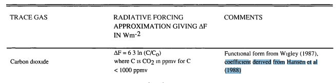
Table 2.2 shows the radiative forcing approximation for CO2:
ΔF = 6.3 ln (C/C0)
With the note:
Functional form from Wigley (1987), coefficient derived from Hansen et al (1988).
viz.:
Hansen et al (1988) is clearly a seminal paper as AR5 referenced Myhre et al. 1998 which also referenced Hansen et al, as well as AR3 referencing it directly.
We are really getting close now! This 1988 paper must be what definitively demonstrated the validity of this radiative forcing calculation approach.
Hansen et al. 1988
This paper is titled “Global Climate Changes as Forecast by Goddard Institute for Space Studies Three-Dimensional Model”.
In the “Introduction” we have:
Studies of the climate impact of increasing atmospheric CO2 have been made by means of experiments [sic!] with three-dimensional (3D) climate models in which the amount of CO2 was instantaneously doubled or quadrupled […] These models all yield a large climate impact at equilibrium for doubled CO2, with global mean warming of surface air between about 2°C and 5°C.
Oh boy… this paper is just yet another model! And not a particularly realistic one either (with CO2 “instantaneously” doubling or quadrupling - later they write their simulation has “no feedback of climate change on ocean heat transport”!). Also note the conflation of running climate models with “experiments” (i.e. control setup done with real life measurements taken).
From section 2. “Climate Model”:
The equilibrium sensitivity of this model for doubled CO2 (315 ppmv → 630 ppmv) is 4.2°C for global mean surface air temperature (Hansen et al. [1984], hereafter referred to as paper 2).
Ok, they refer to an earlier paper of theirs for the equilibrium sensitivity. But how do they know this 1988 or 1984 model reflects realty?
4 Radiative Forcing in Scenarios A, B, C
4.1 Trace Gases
[…]
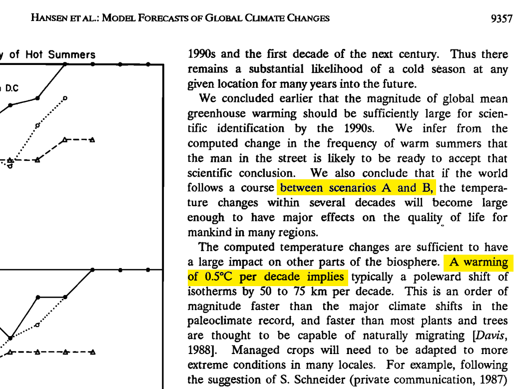
The net greenhouse forcing, ΔT0, for these scenarios is illustrated in Figure 2; ΔT0 is the computed temperature change at equilibrium (t → ∞) for the given change in trace gas abundances, with no climate feedbacks included [paper 2].
[…] we anticipate that the climate response to a given global radiative forcing ΔT0 is similar to first order for different gases, as supported by calculations for different climate forcings in paper 2. Therefore results obtained for our three scenarios provide an indication of the expected climate response for a very broad range of assumptions about trace gas trends. The forcing for any other scenario […] can be compared to these three cases by computing ΔT0(t) with formulas provided in Appendix B.
Ok, this appears sensible. They made a model which is presumed to be accurate by relying on results from an earlier “paper 2”. The model was only run for three specific scenarios, but they provide a formula to interpolate for other scenarios in Appendix B. This latter formula is what appeared in the first IPCC report in 1990.
Let’s first see how the formula is derived, and then we can finally validate all of these calculations empirically!
Appendix B: Radiative Forcings
[…] Radiative forcings for a variety of changes of climate boundary conditions are compared in Figure B1, based on calculations with a one-dimensional radiative-convective (RC) model [Lacis et al., 1981]. The following formulae approximate the ΔT0 from the 1D RC model within about 1% […]
CO2ΔT0(x) = f(x) - f(x0)
f(x) = ln ( 1 + 1.2x + 0.005x^2 + 1.4x10^-6x^3);
x0 = 315 ppmv, x <= 1000 ppmv
Ok, so Hansen et al either created or re-presented a formula to approximate the results of a model from Lacis et al. 1981. This formula was then simplified in AR1 1990 but in a way that preserves the results, presumably.
Let’s see what we find at this 1981 paper…
Lacis et al. 1981
The paper is called “Greenhouse Effect of Trace Gases, 1970-1980”.
Abstract. Increased abundances were measured for several trace atmospheric gases in the decade 1970-1980. […] The combined warming of CO2 and trace gases should exceed natural global temperature variability in the 1980’s and cause the global mean temperature to rise above the maximum of the late 1930’s.
Ok, how do they know?
Observed Trace Gas Abundances
[…] We recognize that more precise future measurements [of our planet’s atmospheric composition] may substantially modify the estimated changes of specific trace gases. Therefore, we give analytic expressions for the computed greenhouse warmings, so the results can be adjusted in accord with more accurate data.1-D Radiative-Convective Model
The 1-d RC model uses a […] The radiative flux is obtained by integrating the radiative transfer equation […] The radiative calculations are made with a method […]
Ok, so it’s just a model with more calculations. How do they know the model is right?
Observed Atmospheric Temperature Trend
Recent analyses agree that the Northern Hemisphere surface air and troposhperic temperatures increased by about 0.1-0.2°C in the 1970’s ([…] Hansen et al., 1981). The latter authors [i.e. Hansen et al.] also analyzed the global mean temperature trend, for which they found a similar increase in the 1970’s.
Normal fluctuations of the smoothed global mean temperature are of the order of 0.1°C for decadal time scales. […] Therefore, although the observed global temperature change in the 1970’s is consistent with that expected from increased trace gas abundances, the change is too small to be confidently ascribed to the greenhouse effect.
Uhm… wow. So the answer is, the author’s of this 1981 paper don’t know that the model calculation reflects reality. They just happened to make a model that matched observed temperatures… that could also be attributed to different things…
Ok, but these calculations matched what Hansen et al found in their “paper 2”. So, this must be where the real evidence lies!
Hansen et al. 1984
This paper is titled “Climate Sensitivity: Analysis of Feedback Mechanisms”.
It should be clear by now that everything relies on this paper’s results. All paths from the most recent AR6 lead backwards towards the 1988 Hansen et al. paper, which is a model that bases the validity of its predictions on this 1984 paper. All the radiative forcing calculations throughout the past four decades rely on the empirical validity of this formula, which so far we have seen only to be based on calculations which one other author indicated could not even account for the calculated effect with certainty.
Everything is on the line here… but as the scientific consensus has been so well-established and peer-reviewed for these past four decades, this must be the rock-hard, firm foundation atop which all of climate science lies!
Abstract. We study climate sensitivity and feedback processes in three independent ways :
(1) by using a three dimensional (3-D) global climate model for experiments [sic] in which solar irradiance S0 is increased 2 percent or C02 is doubled, (2) by using the CLIMAP climate boundary conditions to analyze the contributions of different physical processes to the cooling of the last ice age (18K years ago), and (3) by using estimated changes in global temperature and the abundance of atmospheric greenhouse gases to deduce an empirical climate sensitivity for the period 1850-1980.
Ok, points 1 and 2 are a bit alarming as they are also just models and calculations.
But finally, we get to the nub of the issue! They link the result of the model calculation to an empirically-measured climate sensitivity! Finally we can see how they determined the validity of these calculations.
They detail this 3rd approach here (emphasis mine):
The temperature increase believed to have occurred in the past 130 years (approximately 0.5°C) is also found to imply a climate sensitivity of 2.5-5°C for doubled C02 (f = 2-4). if (1) the temperature increase is due to the added greenhouse gases, (2) the 1850 C02 abundance was 270 +/- 10 ppm, and (3) the heat perturbation is mixed like a passive tracer in the ocean with vertical mixing coefficient k - 1 cm2 s-1.
…
…
…
…
…
And the Oroborous is complete.

…
…
…
WTF !! !! !! !! !! !! !! !! !! !! !!
…
…
…
There you have it. Four decades of research, calculations, models, and scientific consensus around measuring the effect of increased CO2 concentration on global temperature… and it is all based on a 1984 assumption that the (“believed”) temperature rise from 1850-1980 was due to that very effect being calculated, namely increased CO2 concentration (further based upon a starting-point “choice” of one of five values for 1850 CO2 abundance).
There are no further references. The buck stops here. All paths lead to this 1984 paper, which the seminal 1988 paper is based on. The single and solitary validation of the models and calculations reflecting physical reality, proving that increasing CO2 → leads to increasing temperatures in physical reality (and not just in models and calculations), that has been given in these four decades, is that it matches an assumption made in 1984 that an increase in CO2 led to an increase in temperatures.
In other words, the mainstream, scientific consensus is nothing other than forty years of circular reasoning. Each updated report only re-affirms and re-assures that the calculations are established, well-founded, proven effective, and simply refers to earlier works that say the same thing!
Aftermath
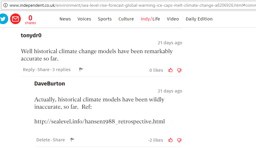
The following article by David A. Burton on sealevel.info is highly informative, titled “Hansen et al 1988, retrospective”:
Reviewing the predictions of a seminal climate modeling paper, thirty years later
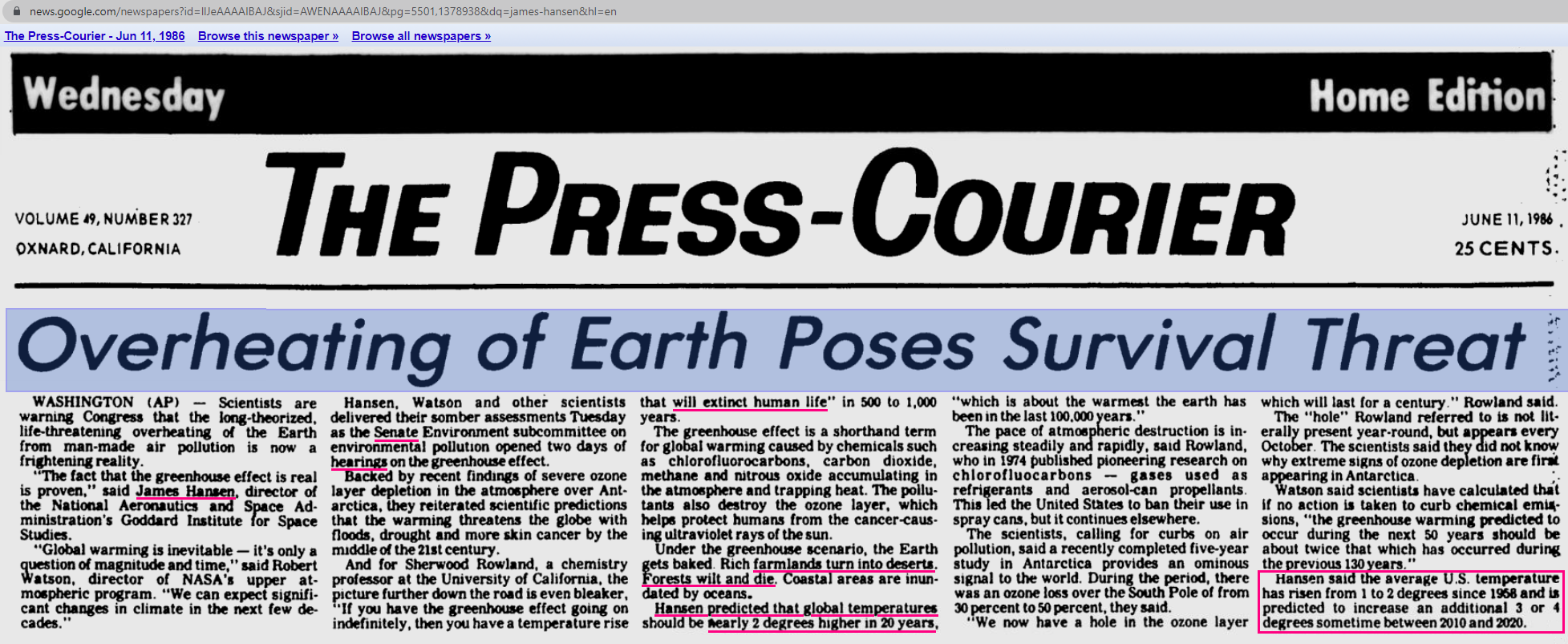
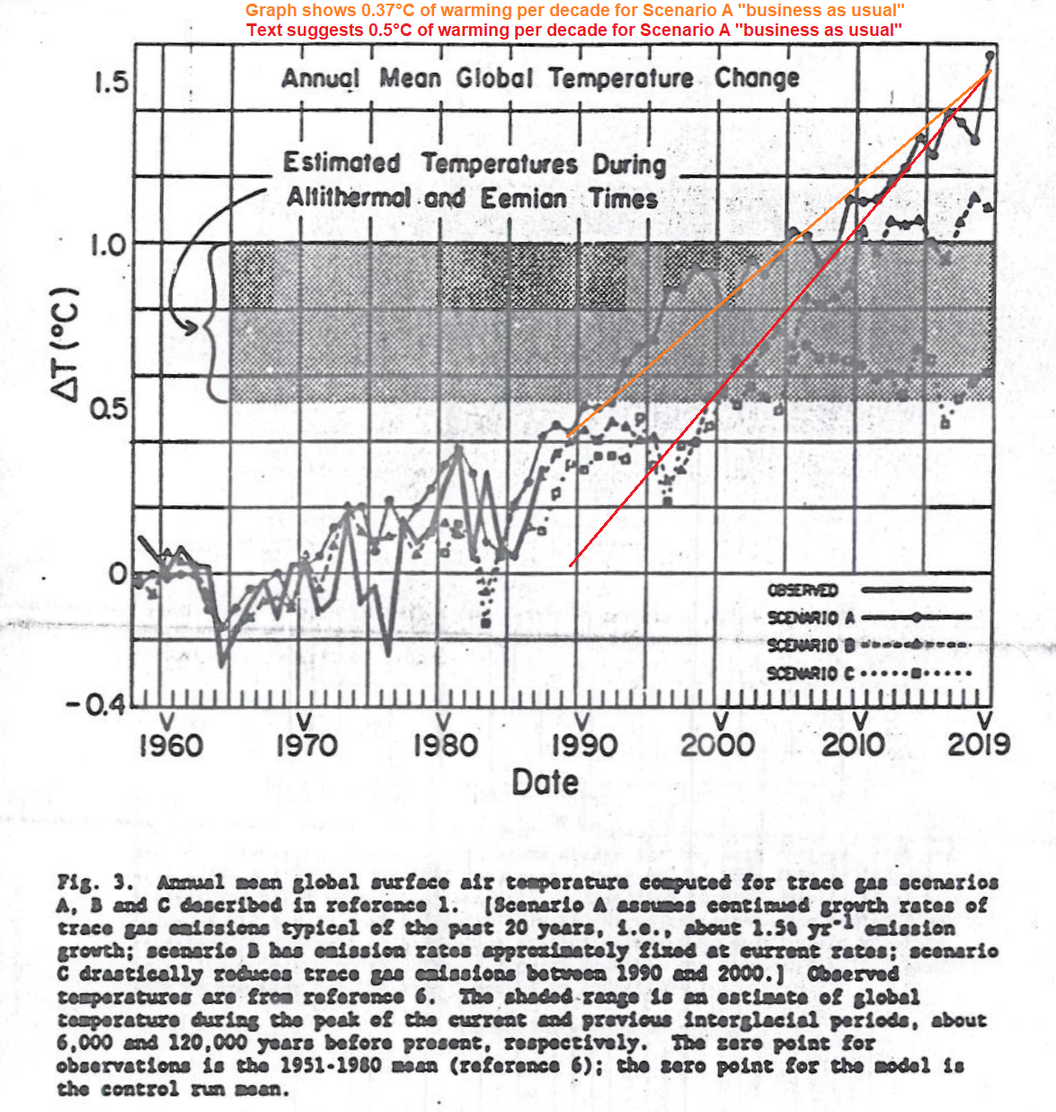
In 1988 NASA’s James Hansen and seven co-authors wrote a highly influential, groundbreaking climate modeling paper entitled, Global Climate Changes as Forecast by Goddard Institute for Space Studies Three-Dimensional Model (pdf). […]
They predicted (src) a “warming of 0.5°C per decade” (or “nearly two degrees F higher in 20 years”) if emissions growth was not curbed (though their graph showed only about 0.37°C per decade).
[…]
Now, I would agree that +0.5°C/decade would be something to worry about! Fortunately, it was nonsense.
[…]
Even so, climate alarmists frequently claim that the NASA GISS model was “remarkably accurate.” Only in the massively politicized field of climatology could a 200% error be described as remarkably accurate. Even economists are embarrassed by errors that large.
[…]
In fact, it wasn’t just their temperature projections which were wrong. Despite soaring CO2 emissions , even CO2 levels nevertheless rose more slowly than their “scenario A” prediction, because of the strong negative feedbacks which curbed CO2 level increases, a factor which Hansen et al did not anticipate. Although CO2 emissions increased by an average of 1.97%/year, CO2 levels increased by only about 0.5%/year.↑
[…]
It is impossible to imagine that Dr. Hansen, his seven co-authors, the peer-reviewers, and the JGR editors, were all ignorant of those already-existing treaties. So there’s no excuse for the paper nevertheless projecting exponential increases in CFCs, in any of their scenarios. They knew CFC emissions would be falling, not rising, yet they promoted a “scenario” as “business as usual,” which they knew was actually impossible.
[…]
In other words, Hansen et al 1988 [i.e. the seminal paper detailed above] was wildly wrong about almost everything.)
Why did they write it, then?
IPCC founded
Most scientists are cautious about making predictions which are apt to embarrass them in the future. But Hansen et al 1988 had a purpose. It was the basis for Dr. Hansen’s famous June 23, 1988 Congressional testimony. 5½ months after that testimony, and 3½ months after the paper was published, the United Nations created the Intergovernmental Panel on Climate Change, to combat the perceived threat — a threat which turns out to have been much ado about very little.↑
?
So, even though the authors got just about everything wrong in their paper, it was nevertheless a great success, because it accomplished what it was intended to accomplish [emphasis added].
Incidentally the following is a very interesting snippet regarding the context of that June 23, 1988 testimony, an excerpt from “The Climate Fix: What Scientists and Politicians Won’t Tell You About Global Warming” (emphasis added):
In the summer of 1988, global warming first captured the imagination of the American public. In early June of that summer Senator Al Gore (D-TN) organized a congressional hearing to bring attention to the subject, one that he had been focusing on in Congress for more than a decade. The hearing that day was carefully stage-managed to present a bit of political theater, as was later explained by Senator Tim Wirth (D-CO), who served alongside Gore in the Senate and, like Gore, was also interested in the topic of global warming. “We called the Weather Bureau and found out what historically was the hottest day of the summer. Well, it was June 6th or June 9th or whatever it was. So we scheduled the hearing that day, and bingo, it was the hottest day on record in Washington, or close to it. What we did is that we went in the night before and opened all the windows, I will admit, right, so that the air conditioning wasn’t working inside the room.”
The star witness that day was Dr. James Hansen, a NASA scientist who had been study climate since the 1960s. […]
Looking back many years later one observer remarked that the 1988 Gore-Hansen hearing in the summer of 1988 “sparked front page coverage across the globe and touched off an unprecedented public relations war and media frenzy, marks the official beginning of the global warming policy debate.” […]
Indeed, Hansen, with his 1984 and 1988 papers, set out to do precisely that which he (along with Al Gore, Tim Wirth, and others) accomplished in 1988, together with a little help of con-artistry of picking the hottest day in summer and turning off the air conditioning during a testimony about global warming: the eventual creation of the IPCC and the birth of a worldwide hoax.
Final Notes
As a final note, the following is relevant when considering the reported historical and recent temperature trends: a series by Jennifer Marohasy titled “Hyping Daily Maximum Temperatures”. It starts as follows:
There is more than one way to ruin a perfectly good historical temperature record. The Australian Bureau of Meteorology achieves this in multiple ways, primarily through industrial scale remodelling (also known as homogenisation – stripping away the natural warming and cooling cycles that correspond with periods of drought and flooding), and also by scratching historical hottest day records, then there is the setting of limits on how cold a temperature can now be recorded and also by replacing mercury thermometers with temperature probes that are purpose-built, as far as I can tell, to record hotter for the same weather.
Cheers,
Claudiu